What’s the Problem?

What is the probability that a protein will be folded at a given temperature? This and many more questions like this are part of statistical mechanics, where we try to describe the average behaviour of many copies of the same system. But how can we compute such probabilities? Simply look at all possible configurations of all folded and unfolded proteins? Sadly, the enumeration of all these states is infeasible, and we therefore have to sample from their equilibrium distribution to compute statistics about the system.

In this blog I present the new approach to generate “one-shot” samples from the paper Boltzmann generators: Sampling equilibrium states of many-body systems with deep learning. With this approach, we can sample from a distribution, whose weights we know, but from which we cannot sample directly. First, I will give an introduction to many-body systems. But I will focus mainly on the machine learning tools they used to achieve this.

Many-Body Problems

Many-body problems are a category of physical problems. They are about microscopic systems made of many interacting particles . The underlying physical laws can be simple, but the resulting system as a whole is extremely complex. In condensed matter physics, the macroscopic and microscopic physical properties of matter are studied, in particular the solid and liquid phases formed by electromagnetic forces between atoms. The system can be described via the equations of motion. The equations thus takes into account the mass, position, energy and forces of the particles. The equations of motion don’t have just one solution, therefore we are talking about probabilities of certain states. Often the most interesting states are rare-events, like the transition of a protein from folded to unfolded or vice versa. One example that we take a closer look at throughout this blog, is an open or closed dimer. This condensed matter system consists of 36 molecules. The focus lies on the two colored particles in figure 1. These can be in two main states: closed (left) or open (right). The transition from one to the other is a rare but interesting event.

closed dimer — Fig.1 Repulsive particle system with bistable dimer. Closed (blue, left), Open (red, right) - F. Noé, S. Olsson, J. Köhler, H. Wu. (2019) [1]

open dimer — Fig.1 Repulsive particle system with bistable dimer. Closed (blue, left), Open (red, right) - F. Noé, S. Olsson, J. Köhler, H. Wu. (2019) [1]

Boltzmann Distribution

The Boltzmann distribution often appears in such problems. It takes into account the energy and temperature of the system. The less energy a state has, the higher its probability is. In our example, the system has the lowest energy, when the dimer is closed or open. To transition from one to the other a high energy barrier must be overcome and therefore these events are quite rare. If we have a given configuration of our system, we can compute the energy and thus can compute the corresponding Boltzmann weight.

Old Approach

The classical approach is to simulate the system. A numerical, iterative solution to the equations of motion is computed with small steps. These steps can be in the order of femto seconds! Therefore, we need a long time to transition from one meta-stable state to the other. For the transition from the open to closed dimer 10¹² simulation steps are needed. Furthermore, the obtained samples are often correlated to each other.

Boltzmann Generators

How can we use machine learning to improve the sampling? As in the name of the paper, Boltzmann generators are used to obtain independent, “one shot” samples. So that we no longer need small simulation steps.

First let’s take a look at what we can do. In our example we have all the positions and forces, for a given sample, between our molecules. We can therefore compute the energy of the system. With this energy we can calculate the Boltzmann weight and know the probability of this state. But we only have no or very few samples. Hence, our problem is sampling.

So how do these Boltzmann generators work? The key idea is a coordinate transformation. From the configuration space X (as seen before: the positions and forces of the molecules) to a so-called latent space Z. There different states are close to each other. And in such a way, that we can sample from there with a Gaussian.

Since in our example this results in a 76 dimensional Gaussian (which is difficult to visualize). Let’s look at a simpler example that shows the principle better:

In figure 2, the left part (blue) shows the configuration space of our data. After the transform we have the samples repacked in a Gaussian like shape (right, blue part). The bends and stretches of the gray lines illustrate well the transformation. Another key part is that the transformation is invertible. That means we can also transform in the other direction. So if we have samples in the latent space (red, right part) we can transform them into our configuration space and get something similar to our data back. In our case we want to draw a sample in the latent space from a Gaussian and then transform the sample to our configuration space to obtain a sample for our original problem.

We do this via a deep invertible neural network. As illustrated in the next image (figure 3):

Sample from Gaussian
Transform via neural network
Reweight

Fig.3 Boltzmann Generators - F. Noé, S. Olsson, J. Köhler, H. Wu. (2019) [1]

We start by drawing a sample from a Gaussian distribution. Then we transform it through our Network and therefore get a sample in our configuration space. We thus generate a distribution p_x. This distribution is similar to the Boltzmann distribution, but not exact. That’s why some reweighting is needed. Our Network consists out of smaller blocks.

Input

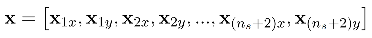
So how does a configuration, and therefore input to our network look like? For our dimer example, we have \( n_s = 36 \) solvent particles and the two dimer molecules. The input vector is simply the alternating x and y position of each particle:

With this input vector we can compute the energy of the system as follows:

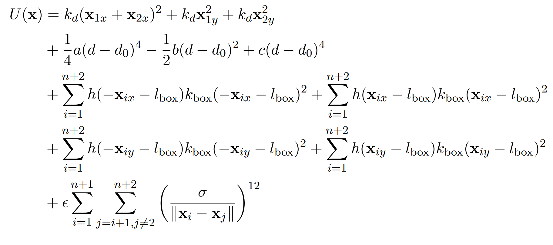
Where \( d = \lVert x_1 - x_2 \rVert \) is the distance between the dimer particles, \( k_d \) is the strength of the bond between the dimer particles, a,b and c are coefficients that describe the energy curve for the dimer, \( d_0 \) is the equilibrium distance between the dimer particles, \( l_{box} \) is the length of the bounding box of the system, \( k_{box} \) is the strength of the bond between the particles and the bound of the box, \( \epsilon \) is the strength of the repulsion between particles, \( \sigma \) is the distance between two particles where the energy between them is zero and h is the step function. The first row are the energy cost of moving the dimer particles in x and y direction. The second row describes the interaction between the dimer molecules. The third and fourth line is for the box constraints on the edges of our system (x and y direction). 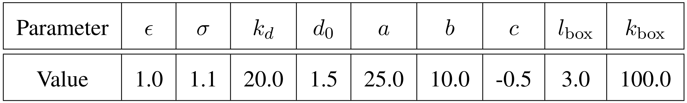And the last row describes the interaction, and therefore repulsion of the other particles. The parameters were chosen as shown in table 1. Therefore, we can compute the energy with this equation for a given sample x. And then, with the energy, we can compute the corresponding Boltzmann weight.

Table 1 Parameters - F. Noé, S. Olsson, J. Köhler, H. Wu. (2019) [1]

Invertible NN

Let’s look at the smaller blocks that make up our network. These blocks are invertible and the Boltzmann generators use RealNVP transformations. It uses only trivial invertible operations, like addition and multiplication. In the image (figure 4), the blue part (left) is for the direction from the latent space to the configuration space and the orange part (right) for the other direction (same in figure 3). First the input is split into 2 channels \( (x_1, x_2) \). One channel remains unchanged and is only used as input to change the second input. S and T are two non-invertible networks. We use the first channel as input of these networks and then multiply or add it to the second channel. Even though the two networks are not invertible, we know their input and therefore can recompute it and then divide or subtract it from the second channel to get our original inputs back. Note that we use the same network both directions. In order to avoid that we only change one half of the input we swap the channel that gets modified every other layer. A block (like \( f_1 \) and \( f_1^{-1} \) in figure 3 ) consist of 2 layers one modification of each channel. We can stack those blocks to obtain a deep neural network. For our running example 8 blocks (with 2 layers each) were used. Furthermore, the networks S and T consist of 3 hidden layers with 200 neurons.

Real NVP Block — Fig.4 Real NVP Transformation Block

Training

Why do we need invertible Blocks? There are two ways to train our network, so that we really get good, realistic samples. And each of it requires the other direction. The first mode is called “training by energy”:

Training by energy

Sample from Gaussian
Transform through NN and generate a distribution p_x

In the beginning p_x will be very different from the Boltzmann distribution. We want to minimize this difference. We therefore use the Kullback-Leibler-Divergence which is derived from the difference between two distributions. So we do not need samples from the configuration space for this training mode. But it tends to focus on the most meta-stable state.

Training by example

Start with a valid configuration (from simulation or experiments)
Transform through NN in other direction

This mode is as we all know training: We start with a valid configuration. This time, we use our transformation in the other direction. “Training by example” is especially good in the early stages, but requires configurations (from experiments or simulations). So the best way is to combine both methods together. For the dimer example, we start with only “training by example” for the first 20 epochs with 10⁵ simulation steps for the open and closed dimer states, but without transitions between these states occurring in the simulations. After that the “training by energy” mode is also used and the whole network is trained for 2000 epochs.

Reweigthing

Because of our network, we never have exactly the Boltzmann distribution. Therefore, we need a bit of reweighting. The third step of the Boltzmann generators. Statistical mechanics offer many tools to generate the wanted distribution when \( p_x \) is sufficiently similar. The easiest way is \( w(x)= \frac{e^{-u(x)}}{p_x} \). Where \( e^{-u(x)} \) is the Boltzmann distribution that we can compute, because we know the energy of the sample. To compute our statistics we use these new weights. And the more equal the distributions are, the better and more accurate the statistics.

Results

Let’s look at the result for the system with the dimer. We recall that the dimer can be closed or open. And these states are separated by a high energy barrier to transition from one to the other. In the latent space, we obtain a 76 dimensional ball. When sampling from a 76 dimensional Gaussian and then transforming it with our (trained) network, we obtain samples, where no particles clash. With these samples we can compute statistic of this system. One possible statistic is the free energy difference. Free energy difference can measure the thermodynamic stability between two states. It is the amount of energy required to transition from one to the other and thus describing the likelihood of a transition. In our case the difference is measured to the state with the lowest energy (closed state). In the following image (figure 7) this difference is plotted against the distance of the dimer particles. The black line was obtained by classical sampling methods. The green points are samples generated with the Boltzmann generators, which are very close to the black line. The intervals around some green points are the standard errors from 10 independent repeats.

Fig.7 Free Energy Difference - F. Noé, S. Olsson, J. Köhler, H. Wu. (2019) [1]

For one transition from one meta-stable state to the other and back, the simulation needs 10¹² steps. To get the same precision as the Boltzmann generators we need 100 of those transitions. On the other hand the Boltzmann generators need 2*10⁷ energy evaluation in the training process. This is a significant speed-up by 7 orders of magnitude! In addition, the samples are independent and “one-shot”. That means we can draw as many samples as we want without significant computations.

Transition Paths

What else can we do with the transformation? If we take our 2 meta-stable states, we can do a linear interpolation in the latent space. If we transform this path back to the configuration space, we obtain possible and realistic transition paths from one to the other. One of these paths can be seen in the next image (figure 8).

Conclusion

We can use the Boltzmann generators for rare-event sampling problems in many-body systems. Furthermore, we obtain independent one-shot samples. And in the paper they show an example with a dense systems with more than 1000 dimension. But the approach is not ergodic, which means it does not cover the whole configuration space. Although in the paper some ideas are brought up to combine the Boltzmann generators with classical sampling methods to fix this. Moreover, the networks are always very system specific, and therefore we have to train on every configuration space from scratch. Ideally we could pretrain the Boltzmann generators so that we only have to fine-tune it to every special use case. We also end up with the trade off that we do not have to do the small simulation steps, but the more complex the system the more difficult it is to reweight and the results are not that accurate anymore. The Boltzmann generators can be used in many topics and there are some papers that build up on it. So whenever we want to sample from a known distribution we can use this approach. A short summary of the most important take-away points:

Statistical mechanics aims to compute statistics about a many-body system, which can have a huge configuration space, and we therefore need to sample
The Boltzmann distribution describes the probability of a configuration given the energy
But we can use this approach also when we want to sample from a (any) known distribution
The traditional approach uses tiny simulations steps, which are computationally expensive and the obtained samples can be correlated
Boltzmann generators are a new approach that uses machine learning to obtain independent “one-shot” samples
The key idea is a coordinate transformation to a latent space, where different states are close to each other so that we can sample from a simple Gaussian distribution
These samples can then be transformed back to the configuration space to obtain valid samples for the system

References

[1] F. Noé, S. Olsson, J. Köhler, H. Wu; Boltzmann generators: sampling equilibrium states of many-body systems with deep learning; Science, 365 (2019)
[2] Dinh, Laurent, Jascha Sohl-Dickstein, and Samy Bengio. “Density estimation using real nvp.” arXiv preprint arXiv:1605.08803 (2016)
[3] Frank Noe. (2020, 26. September). MLDS 2020 - 3 Boltzmann Generators. YouTube. https://youtu.be/WuXJRswYIaA
[4] ICTP Condensed Matter and Statistical Physics. (2021, 16. December). Enhanced sampling in Molecular Dynamics: Why is it necessary?. Youtube. https://www.youtube.com/watch?v=2S3xYRLy2cI